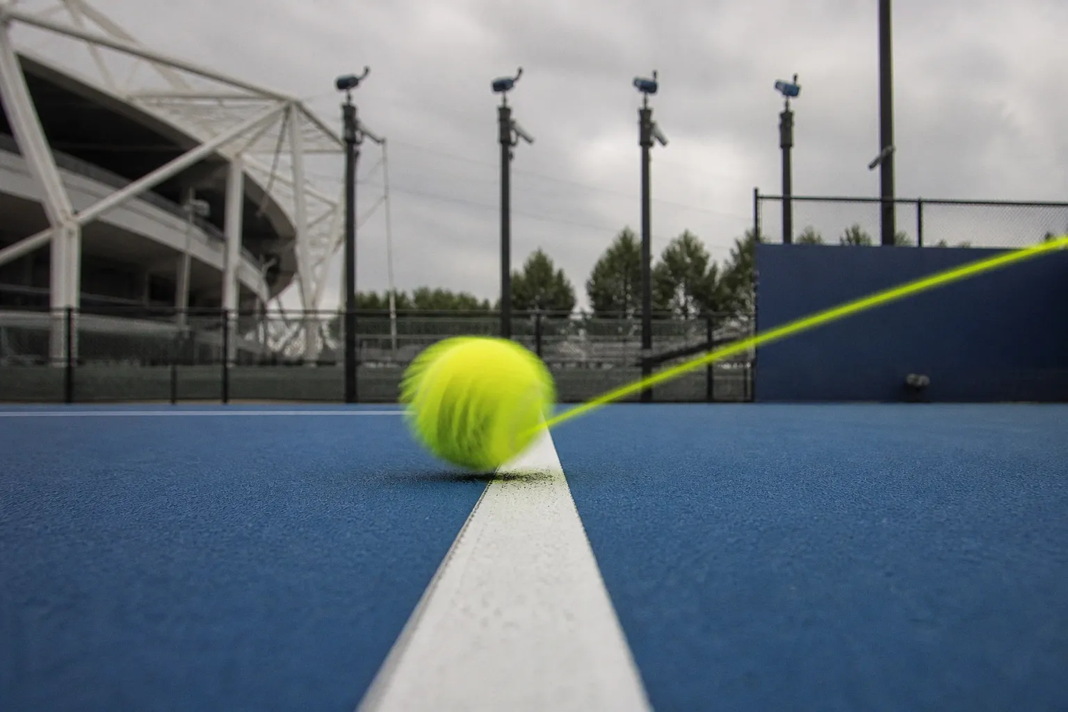
That is not enough to make the system unreliable. It is enough to make the word infallible mathematically incorrect.
The hawkeye margin of error in tennis line calls is small relative to the court. It is not small relative to the event being measured. A line call is often decided by a few millimeters. The system is reconstructing the position of a fast, deforming object at the instant it contacts a surface. It is not reading a photograph.
From optical illusion to digital reconstruction
Hawk-Eye does not record a high-definition image of the ball touching the court and then enlarge the relevant pixels. The system uses multiple high-speed cameras to observe the ball from different angles. It then triangulates the recorded positions and calculates a three-dimensional trajectory.
The output is a model.
The standard camera array can include up to 10 high-performance cameras positioned around the court. Each camera supplies two-dimensional observations. The system combines them to estimate the ball’s path through three-dimensional space. It then projects the calculated trajectory onto the court plane and renders the bounce.
The displayed animation is therefore a visual representation of data. It is not direct evidence of the physical mark left by the ball.
That distinction matters because a tennis contact is not a clean geometric event. The ball changes shape. The court surface compresses. The ball can skid after contact. Clay can preserve a mark that extends beyond the point used by the tracking model. Hard courts usually provide no visible mark for comparison.
The system is solving several problems at once:
- locating the ball in each camera frame;
- synchronising the cameras;
- reconstructing the ball’s three-dimensional position;
- estimating the trajectory between observed points;
- modelling the bounce and its relationship to the court surface;
- determining whether the ball intersects the legal boundary.
The final call depends on the calculated position of the ball relative to the line. It does not depend on one camera producing a perfect image.
Hawk-Eye does not remove uncertainty. It converts uncertainty into a quantified geometric estimate.
The court itself is easier to define than the ball. Court lines have fixed locations. The ball does not. Its centre, edge, compression, skid and camera visibility all affect the calculation. The closer the bounce is to a line, the more significant those variables become.
This is why the rendered image can look precise while the underlying decision still has a measurable error range. A clean graphic does not mean that the physical event was observed with zero uncertainty.
The 2.6 millimeter reality
The most useful figure in the available testing data is the 2.6 mm mean absolute error recorded in ITF testing. Other official figures place Hawk-Eye’s average margin of error between 2.2 mm and 3.6 mm.
The word mean is doing technical work here.
A mean absolute error is an average of the absolute differences between the system’s calculated position and the reference position. It does not state that every call is wrong by exactly 2.6 mm. It does not establish a fixed circular zone around every bounce. It does not mean that the system can be off by only 2.6 mm in every direction and under every condition.
The value describes system performance across a set of tests. Individual observations can sit closer to the reference position or farther from it.
The relationship between the error figure and the ball is also useful. An ITF-approved standard tennis ball has a diameter of 67 mm. A 2.6 mm mean error is approximately 3.9% of the ball’s overall diameter. At the upper cited figure of 3.6 mm, the ratio is approximately 5.4%.
That comparison does not mean the whole ball is misplaced by 5.4% in every call. It shows the scale of the uncertainty against the object being tracked.
| Measurement | Value | What it describes |
|---|---|---|
| Standard tennis ball diameter | 67 mm | Overall width of the ball |
| ITF mean absolute error | 2.6 mm | Average absolute difference in testing |
| Lower cited Hawk-Eye margin | 2.2 mm | Reported average error range |
| Upper cited Hawk-Eye margin | 3.6 mm | Reported average error range |
| Upper margin as share of ball diameter | About 5.4% | Scale comparison, not a per-call probability |
A line is not a point. It has width. The legal question is whether any part of the ball overlaps the boundary. The system therefore needs to estimate the ball’s position and the contact geometry relative to the court marking.
If the estimated bounce is well inside the court, a few millimeters of error do not change the result. If it is well outside, the same applies. The difficult cases are concentrated near the boundary. That is where the error interval intersects the decision threshold.
This is a classification problem. The system is not asked to provide an abstract coordinate. It is asked to convert a coordinate estimate into one of two outcomes: in or out.
The closer the estimate is to the boundary, the less separation exists between those outcomes.
Mean error is not the same as certainty
A common misunderstanding treats the quoted number as a guarantee. If the margin is 2.6 mm, the reasoning goes, every call within 2.6 mm must be uncertain and every call beyond it must be correct.
That is not how the figure works.
A mean error is a performance summary. It is not a universal tolerance band. It does not disclose every component of the system’s uncertainty, and it does not turn the graphic into a laboratory measurement for an individual bounce.
The error can be influenced by several factors:
- camera angle and the visibility of the ball;
- the number of cameras contributing useful observations;
- image quality and calibration;
- the timing of the frames used for trajectory reconstruction;
- the speed and spin of the ball;
- the geometry of the bounce;
- ball deformation at contact;
- surface behaviour after impact.
The available public facts do not establish one universal error figure for every court, camera configuration and environmental condition. They also do not provide the proprietary source code or the full modelling procedure used for skid and compression on different surfaces.
That limits what can responsibly be claimed. The system is highly accurate. It is not perfect. The quoted millimetres are averages, not a promise attached to every individual call.
Ball compression and surface skid
The ball does not remain spherical when it hits the court.
At contact, the felt and rubber deform. The court surface may compress. The ball’s vertical velocity changes. Its horizontal velocity may not disappear. Depending on the angle, spin and surface, the ball can slide or skid before the bounce is fully resolved.
This creates several different positions that are easy to confuse:
1. the position of the ball’s centre before contact;
2. the point at which the ball first intersects the court plane;
3. the area of the ball in contact with the surface;
4. the visible mark produced after the ball has moved across the surface;
5. the position represented by the Hawk-Eye reconstruction.
These positions are related. They are not necessarily identical.
On clay, a player may inspect a mark that appears to show the physical contact. Even there, the mark is affected by compression and lateral movement. The visible imprint can be elongated or displaced relative to the initial point of contact. Hawk-Eye’s rendered bounce is based on trajectory calculations. It is not a scan of that mark.
On hard courts, the same physical event produces no comparable imprint. The tracking system becomes the primary measurement method rather than a digital comparison to visible evidence.
The difference between a mark and a model does not automatically indicate a system failure. It indicates that two methods are measuring different representations of the bounce. One records a disturbance in the surface. The other estimates a trajectory and its intersection with the court.
Why a close call can look wrong
A rendered animation often creates an impression of visual certainty. The replay shows a ball and a line. The image appears final. But the ball shown on screen is not a captured frame with independently visible edges. It is a computed object placed on a computed trajectory.
The graphic is designed to communicate the result quickly. It is not designed to display a confidence interval or a probability distribution. Viewers see a boundary decision. They do not see the camera calibration, the triangulation residuals or the model’s assumptions about the bounce.
This is a presentation issue, not necessarily a technical defect.
A system can make a correct classification while using a position estimate with non-zero error. It can also make an incorrect classification even when the average system performance is very strong. The average says how the system performs across tests. It does not settle every case at the line.
The practical distinction is simple:
- a clear in call has a large geometric separation from the boundary;
- a clear out call has a large separation in the opposite direction;
- a line call sits close to the decision boundary and is more sensitive to small changes in the estimated trajectory.
The third category is where the hawkeye tracking system limit in tennis becomes visible. Not because the system suddenly stops working. Because the classification threshold is narrow.
The evolution of electronic line calling
Hawk-Eye first appeared in professional sport as a broadcast technology. Its first implementation was in cricket in 2001. Tennis adopted the challenge system officially in 2006.
The original challenge format placed the technology inside a human decision structure. A player disputed a line call. The system supplied a review. The umpire then applied the result under the competition rules.
This created a specific use case. Hawk-Eye did not need to replace every line judge. It needed to provide a sufficiently accurate adjudication mechanism when a call was challenged.
That system changed the role of the displayed reconstruction. The animation was not only a broadcast feature. It became the public-facing explanation of a ruling. The audience saw the model, and the model became associated with finality.
Fully automated Electronic Line Calling, or ELC Live, removes the challenge step and supplies calls in real time. It debuted at the Next Gen ATP Finals in 2018. The technology therefore moved from retrospective verification toward continuous officiating.
The mathematical problem remained. Automated line calling still depends on cameras, calibration, trajectory reconstruction and a court model. The system’s authority increased, but its physical measurements did not become exact merely because the calls were automated.
| System role | Human process | Technical output | Main implication |
|---|---|---|---|
| Challenge review | Player requests a review | Reconstructed bounce and ruling | Used to check a disputed call |
| Automated ELC | System calls the ball live | Real-time line decision | Removes the line judge from the call |
| Broadcast graphic | Viewer sees the result | Rendered 3D animation | Communicates the model, not a photograph |
The transition also changes how errors are experienced. Under a challenge system, only selected calls are exposed to review. Under live electronic calling, every decision is generated by the system. A rare borderline error can therefore become more consequential if it occurs at a break point, on a second serve or during a long rally.
That consequence is competitive. It does not mean the technical error rate has increased. It means the system’s output is now embedded directly in the point sequence.
When the margin meets the boundary
The most useful way to interpret electronic line-calling accuracy statistics is through decision geometry rather than absolute confidence.
Suppose a trajectory estimate places the ball several centimetres inside the court. A 2.6 mm average error is not operationally significant. The estimated contact point remains inside under ordinary deviations of that scale.
Now suppose the estimate places the ball 1 mm outside the line. The average error is larger than the distance to the boundary. The call is sensitive to the reconstruction. A small shift in the estimated trajectory could move the calculated contact from outside to inside.
This does not produce a simple rule that every call within 2.6 mm is undecidable. The margin is not a court marking. It is not a mandatory buffer. It is a statistical property of system performance.
The correct question is not whether the line call lies inside an abstract error circle. The correct question is how far the estimated contact is from the boundary relative to the known uncertainty of the system and the specific geometry of the bounce.
In simplified form:
- large separation from the line reduces classification sensitivity;
- small separation from the line increases classification sensitivity;
- zero apparent separation creates the maximum dependence on the reconstruction model.
The system also needs to account for the rule that the ball is in if any part of it touches the line. That makes the relevant geometry different from tracking only the ball’s centre. The ball’s diameter, deformation and contact point matter.
A 67 mm ball can overlap a line even when its centre is not directly above the painted boundary. Conversely, a rendered point can appear near a line without showing the full physical interaction between ball, surface and marking.
This is why the visual gap in a replay should not be interpreted as a direct millimetre ruler. The animation communicates the calculated result. It does not expose all the underlying geometry.
The line is binary. The measurement is not.
Why the system remains useful
A non-zero error margin does not undermine the purpose of Hawk-Eye. It defines the limits within which the system should be interpreted.
Human line judges also operate under uncertainty. They observe a fast event from a fixed position, often with partial occlusion and limited reaction time. Hawk-Eye replaces that judgment with a calibrated multi-camera reconstruction. The comparison is not between perfect and imperfect observation. It is between different sources of error.
The system’s advantage is consistency and scale. It can process trajectories across the court using the same measurement framework. It can make a live call without relying on one official’s viewing angle. It can also provide a review mechanism that is more systematic than a replay selected for television.
The correct conclusion is narrower than complete infallibility and stronger than general suspicion:
Hawk-Eye is accurate enough to serve as an official line-calling system, but its accuracy has a measurable physical limit. The typical quoted margin is measured in millimetres because the decision itself is measured in millimetres.
What the number tells us about future tennis
The development from challenge review to automated ELC will continue to move officiating toward machine-generated decisions. The strategic effects will be indirect but real.
Players already treat line-calling systems as part of the court environment. Serve placement, return position and rally tolerance are built around narrow margins. A server targeting the outside edge of the service box is not operating in the same geometric space as a player hitting through the middle. The official system determines whether those margins are converted into points.
The technology may become faster, more integrated and less visible. That will not eliminate the underlying problem. Every system that tracks a physical ball must estimate position from observations. Every estimate has uncertainty.
Future improvements can reduce the mean error. Better camera calibration can reduce reconstruction noise. More consistent court conditions can reduce modelling variation. More detailed surface models may improve the relationship between the calculated bounce and the physical event.
None of these changes creates a zero-error system. They move the threshold.
The important data point is therefore not only the headline number of 2.6 mm. It is the relationship among:
- the ball’s diameter;
- the distance between the estimated contact and the line;
- the geometry of the bounce;
- the surface response;
- the camera observations available to the reconstruction;
- the rule used to classify contact with the boundary.
A single average cannot describe all of those variables. It can establish scale. Hawk-Eye’s mean error is measured in a few millimetres. The tennis ball is measured in tens of millimetres. The boundary between a point won and a point lost can be narrower than both.
The final calculation
The hawkeye margin of error in tennis line calls is not evidence that electronic officiating is arbitrary. It is evidence that electronic officiating is a measurement system.
Hawk-Eye uses multi-camera trajectory triangulation. It can rely on up to 10 high-speed cameras. It generates a simulated 3D bounce. It does not display a photograph of the ball touching the court. Its officially cited average error range is 2.2 mm to 3.6 mm, with an ITF mean absolute error of 2.6 mm.
That is a strong level of accuracy. It is not absolute accuracy.
For clear calls, the difference is irrelevant. For a ball near the boundary, it is the entire problem. The closer the estimated contact is to the line, the more the result depends on the quality of the trajectory reconstruction and the assumptions applied to ball contact.
The scoreboard still records a binary outcome. The court does not. Between in and out sits a small but measurable field of uncertainty. Hawk-Eye narrows that field to millimetres. It does not remove it.